This guest article was written by Nicolas Tröger. Nicolas is a software developer and computer science student specializing in software engineering, cloud, virtualization, and IT security. He has also gained hands-on experience in data engineering, particularly in building data pipelines and working with open data.
What This Post Covers
- How data engineering is essential to make (open) data usable (e.g. data analysis)
- How data engineering can be done in general and the use-cases for domain-specific languages (DSL)
- Step-by-step walkthrough of an ETL pipeline using Jayvee, a DSL:
- Extracting from local and online sources
- Transforming messy data into structured tables
- Loading cleaned data into a SQLite database
- Practical example of processing data: U.S. storm casualty data + climate opinion data.
This is the second post in a series on using open data for real-world impact – from climate research to disaster response. While open data holds tremendous potential, it’s often held back by inconsistent formats, poorly documented structures, and minimal preparation by data publishers. In many cases, datasets are released simply to meet legal requirements, not out of a genuine commitment to transparency or usability.
This is where data engineering becomes essential. It’s the discipline of designing and managing workflows that transform data into usable, structured information – and for open data, it’s often the first critical step before analysis can even begin.
There are countless tools for working with data, ranging from general-purpose programming languages (GPLs) like Python to no-code, UI-based platforms for assembling data pipelines. The latter are often praised for their accessibility – especially for users without a programming background. But as open data reaches a broader and more diverse audience, it’s worth asking: Why not just stick with visual or no-code tools?
The short answer: scalability, reproducibility, and openness. UI-based tools often struggle with version control, automation, and integration into collaborative workflows – especially in larger projects. Many are also proprietary, limiting transparency and long-term sustainability. In contrast, programmable / text-based approaches (like those used in GPLs) integrate well with established tools like version control systems (e.g. Git), support automation, and encourage reproducible results.
Still, GPLs can be complex and intimidating for newcomers.
That’s where domain-specific languages (DSLs) come in – lightweight languages designed for a particular task. They aim to strike a balance between the accessibility of visual tools and the power and structure of programming languages. One such DSL is Jayvee, designed specifically for creating data pipelines in a readable and structured way. It supports automation and reproducibility, and it’s significantly easier to learn than full-blown programming languages.
What is data engineering?
Data engineering applies software engineering principles to design and build data infrastructure that supports the collection, processing, and organization of data. This foundation is crucial for enabling downstream tasks such as analytics or machine learning and often requires handling large-scale storage, computation, and data transformation workflows.
One large part of professional data engineering is managing and building automated data pipelines with ETL (Extract, Transform, Load) being the most common form of pipelines. This is a process that extracts data from sources, transforms it into usable format and loads it into storage systems. For that purpose, ETL-Pipelines are used, which are designed and implemented by data engineers. These pipelines can often come together with automation and reproducibility. They can be created by using general-purpose programming languages like Python or Java, aswell as dedicated DSLs and tools to create such pipelines.
Summary of ETL-Pipelines:
- Extract: Data is gathered from diverse sources like databases, APIs, or files.
- Transform: The extracted data is cleaned, standardized, and converted into a consistent format suitable for analysis. This often involves filtering, aggregating, and joining data.
- Load: The transformed data is then loaded into a target system, such as a data warehouse or data lake, for storage and further use.
We’ll walk through these steps using a practical example built with a Jayvee pipeline. The data sources include records of storm-related casualties and survey data on public agreement with climate change countermeasures across U.S. states. For more background on how these datasets were selected, see the (first post in this series).
What’s Jayvee?
Jayvee is a text-based domain-specific language tailored for data engineering. It’s used for automated processing of data pipelines and is fully open-source. One of its goals is to enable collaboration with subject matter experts that might not be professional programmers by focusing on data engineering concepts and the self-explanatoriness of the written Jayvee code, supported by clear documentation. It can be used to extract data, which can be preprocessed/transformed (e.g., cleaning) and loaded into suitable data formats (e.g., different data format than the input format).
An installation guide can be found here.
Once installed, a pipeline can be run with “jv example.jv” with example.jv being a .jv-textfile in which a pipeline is declared with basic human-readable text.
Practical Example: Extracting data
As a first step, we need to handle data extraction. Data used as input for pipelines can be, for example, databases, APIs, files, or web services. One common approach is looking for a download link of a dataset while searching for the data. It is important that the download link is as stable as possible to ensure reproducibility (e.g., same dataset behind the URL, no broken links).
To show the data extraction with Jayvee, we first need to introduce how to generally write down Jayvee pipeline code.
The code below shows two larger blocks marked with the keyword pipeline and a name. These are the actual pipeline elements wrapping all the code that will be defined for a pipeline execution. In total, we can see two pipelines defined in the same file, which will be executed independently. A pipeline is a sequence of different computing steps – the blocks. The order of the blocks being executed is given by the pipe notation (e.g., WeatherExtractor -> WeatherTextFileInterpreter). These also define which output of a prior block gets sent as input to the following block.
// Pipeline 1
pipeline WeatherPipeline {

    WeatherExtractor
        -> WeatherTextFileInterpreter;

    ...
}


// Pipeline 2
pipeline PoliticalOpinionPipeline {

    PoliticalOpinionExtractor
        -> PoliticalOpinionTableInterpreter

    ...
}
Now let’s start by writing down the contents of our pipeline. Jayvee has many different blocks to configure how data should be computed. We won’t discuss all of them – just the ones we are actually going to use. For more details, see the mentioned documentation. But just to grasp how a pipeline should be structured in terms of computing steps, here is a quick overview of the blocks:
- Extractor: Blocks that model a data source.
- Transformator: Blocks that model a transformation.
- Loader: Blocks that model a data sink.
The general structure of a pipeline consisting of different blocks is the following:

The common syntax of blocks is, at its core, a key-value map to provide configuration to the block. The availability of property keys and their respective value types is determined by the type of the block, called the block type – indicated by the identifier after the keyword oftype. Each block can have a customized name.
As the block type of our extractor block in the first pipeline suggests, a LocalFileExtractor is an extractor that picks up locally existing files under the configured path and filename and makes them available for our pipeline.
Note: This block can pick up local files, but since our weather data is compressed as a .gz file and Jayvee doesn’t support decompression yet, we use a shell script to download, decompress, and save the file locally. Another script runs this and then starts the pipeline, ensuring reproducibility without dependency issues.
// Pipeline 1
    ...

    block WeatherExtractor oftype LocalFileExtractor {
        filePath: "weather_events.csv";
    }

    ...
The second block is a “CSVExtractor” that downloads a arbritrary file by the configured download url. Additionally, you can configure which delimiter should be used to separate the values in the .csv file. This can differ – for example, some formats use a semicolon as a delimiter. The enclosing character for values can also be configured, which specifies the character used to wrap values. All of this can to be identified by viewing the CSV file in raw text format and adjusted in the pipeline accordingly.
The CSVExtractor is a composite block and available in the standard library. You can build your own blocks out of existing built-in blocks to, for example, combine certain related steps.
// Pipeline 2

    ...

    block PoliticalOpinionExtractor oftype CSVExtractor {
        url: "https://raw.githubusercontent.com/yaleschooloftheenvironment/Yale-Climate-Change-Opinion-Maps/refs/heads/main/YCOM5.0_2020_webdata_2020-08-19.csv";
        delimiter: ",";
        enclosing: '"';
    }

    ...
For the local file extraction of the first pipeline, there is no ready-to-go block, so the basic built-in blocks will be used for converting the downloaded file to a csv file (TextFileInterpreter and CSVInterpreter). They will be used to interpret the file in terms of delimitation and enclosings.
Whether we do it with the CSVExtractor or the basic blocks, we will end up with a virtual csv file that can be handled further by the pipeline.
Data Transformation
Once data is extracted, it’s often messy, inconsistent, or incomplete – especially in the world of open data. That’s where data transformation comes in: the step in ETL pipelines that turns raw inputs into clean, structured, and analysis-ready formats.
Transformation ensures data is consistent, interpretable, and meaningful. Without it, downstream tasks like visualization or data analysis become unreliable or even impossible.
The transformation stage typically involves a series of steps that clean, standardize, and reshape the data:
1. Format Conversion and Parsing
Open data can come in various formats like CSV, JSON, or Excel. One of the first tasks is parsing these into a structured internal format – like a table or dataframe. This often involves flattening nested data (e.g., JSON) or extracting fields from unstructured text. In our case, we already did that with out CSVExtractor.
2. Encoding and Type Normalization
Text data may use inconsistent character encodings (e.g., UTF-8 vs. ISO-8859-1). Unifying encodings ensures special characters display correctly. At the same time, data types (like numbers or dates) often need to be coerced from raw strings into usable formats.
3. Cleaning and Fixing
Cleaning tackles problems like missing values, duplicates, or formatting issues. This may involve:
- Replacing or imputing missing entries
- Standardizing formats (e.g., date or number styles)
- Correcting typos or inconsistent labels. It’s also common to filter out corrupted or incomplete rows at this stage.
4. Filtering and Subsetting
Often, only a portion of the dataset is relevant. Filtering helps remove noise – for example, by selecting specific columns, excluding outliers, or focusing on one region or time period.
5. Deriving New Data
Transformations can also include calculating new fields from existing ones – like computing averages, rates, or classifications. For example, you might calculate a “storm severity score” or group age ranges into broader categories.
6. Validation
Before loading data into a target system, it’s good practice to validate it: check that required fields are present, values fall within expected ranges, and formats match expectations.
Practical Example: Transforming data
1. Pipeline:
Example of data structure:
| … | STATE | … | INJURIES_DIRECT | INJURIES_INDIRECT | DEATHS_DIRECT | DEATHS_INDIRECT | … |
|---|---|---|---|---|---|---|---|
| … | GEORGIA | … | 3 | 0 | 0 | 0 | … |
| … | KANSAS | … | 0 | 0 | 0 | 8 | … |
| … | KANSAS | … | 0 | 3 | 0 | 0 | … |
| … | KANSAS | … | 5 | 0 | 0 | 0 | … |
| … | COLORADO | … | 0 | 0 | 0 | 0 | … |
| … | COLORADO | … | 0 | 0 | 5 | 0 | … |
| … | KANSAS | … | 6 | 0 | 0 | 0 | … |
| … | COLORADO | … | 102 | 0 | 0 | 0 | … |
With our extraction step we ended up with a csv file that can be interpreted as a table, which will be done almost automatically by defining whether there is a header row present (in most cases, the first row of the CSV dataset), as well as what columns are present. If a header row is present, the columns between the original headers and the Jayvee-code-defined column names will be matched; otherwise, the virtual table will assign column names in order to the original columns.
By using column names that already exist, we can specifically define only certain columns to be used in our virtual table and therefore eliminate irrelevant columns, reducing the data size. You also define the most fitting data type, which can be integer, text (string-like), decimal, or boolean.
    block WeatherTableInterpreter oftype TableInterpreter {
        header: true;
        columns: [
            "STATE" oftype text,
            "INJURIES_DIRECT" oftype integer,
            "INJURIES_INDIRECT" oftype integer,
            "DEATHS_DIRECT" oftype integer,
            "DEATHS_INDIRECT" oftype integer
        ];
    }
Now, this virtual table will serve as the base for performing transformations.
A transformation can be performed by declaring a TableTransformer block, where we define the input columns (names explicitly given in the TableInterpreter block) and specify an output column. If the output column has the same name as an existing one, it will be overwritten; otherwise, a new column will be created and added to the table. The transformation is defined by configuring which transform block it uses and will be performed for each row using the values defined in the inputColumns field.
In our case, we let Jayvee create a new column, since we want to store values that don’t exist in the original dataset – specifically, the sum of the prior input columns.
The transform block then defines, using ports, how to provide the input values as variables that can be used in assignments. This example shows how we output a value for each row using the TotalCasualties output port, which will populate the new TOTAL_CASUALTIES column.
The “TotalCasualties:” line signals what value is assigned to that output port, and consequently, the values in the resulting column. In our case, it’s a simple sum calculation.
    block CasualtiesTransformer oftype TableTransformer {
        inputColumns: [
            "INJURIES_DIRECT",
            "INJURIES_INDIRECT",
            "DEATHS_DIRECT",
            "DEATHS_INDIRECT"
        ];
        outputColumn: 'TOTAL_CASUALITIES';
        uses: TotalCasualties;
    }

    transform TotalCasualties {
        from Injuries_dir oftype integer;
        from Injuries_ind oftype integer;
        from Deaths_dir oftype integer;
        from Deaths_ind oftype integer;
        to TotalCasualties oftype integer;

        TotalCasualties: Injuries_dir + Injuries_ind + Deaths_dir + Deaths_ind;
    }
Overview of data after transformations:
| STATE | INJURIES_DIRECT | INJURIES_INDIRECT | DEATHS_DIRECT | DEATHS_INDIRECT | TOTAL_CASUALITIES |
|---|---|---|---|---|---|
| GEORGIA | 3 | 0 | 0 | 0 | 3 |
| KANSAS | 100 | 212 | 0 | 8 | 312 |
| KANSAS | 0 | 3 | 0 | 0 | 3 |
| KANSAS | 5 | 0 | 0 | 0 | 5 |
| COLORADO | 0 | 0 | 0 | 0 | 0 |
| COLORADO | 0 | 0 | 5 | 0 | 5 |
| KANSAS | 6 | 0 | 0 | 0 | 6 |
| COLORADO | 102 | 0 | 0 | 0 | 102 |
2. Pipeline:
Example of data structure:
| GeoType | GeoName | CO2limits | fundrenewables | … |
|---|---|---|---|---|
| State | Wyoming | 70,49 | 85,49 | … |
| County | Houston County, Alabama | 45,6 | 32,45 | … |
| State | Kansas | 33,45 | 68,98 | … |
We already know how the TableInterpreter works; the only specialty now is that for the column “GeoType” the data type is “State,” which is none of the previously mentioned ones. This is because, besides the built-in types we discussed, there are also primitive types. These are custom types consisting of built-in data types but with customized constraints that rows and their corresponding values need to fulfill. This way, you can define an original column as an integer column but specify that the allowed values are only between 0 and 100 (e.g., defining a 0-100% range). All rows with values in that column that don’t fit the constraint will be excluded. This allows you to filter your data.
The custom type can be defined by declaring a valuetype with a name and the underlying built-in type. Then we declare an array of constraints.
These constraints are based on a Jayvee built-in constraint type (in our case, AllowlistConstraint), each having different functionality. In our case, we have an allowlist to which we provide one or multiple text strings that will be matched with the values. If they match, the constraint is fulfilled. Since this is our only constraint, it means each value of a row in that column must match the text “State”; otherwise, the row is removed. In our case, the column GeoType can also have text values like “County,” so only the rows flagged as “State” will remain in the table.
    block PoliticalOpinionTableInterpreter oftype TableInterpreter {
        header: true;
        columns: [
            "GeoType" oftype State,
            "GeoName" oftype text,
            "fundrenewables" oftype decimal,
            ...
        ];
    }

    valuetype State oftype text {
        constraints: [
            StateFilter,
        ;
    }

    constraint StateFilter oftype AllowlistConstraint {
        allowlist: [
            "State",
        ];
    }
In similar manner to the first pipeline, we perform transformations like creating a new column with a newly calculated average value per row or transforming the content of the GeoName column to uppercase.
Overview of data after transformations:
| GeoType | GeoName 2 | CO2limits | drilloffshore | … | AverageOpinionTrend |
|---|---|---|---|---|---|
| State | WYOMING | 70,49 | 85,49 | … | 77,99 |
| State | KANSAS | 33,45 | 68,98 | … | … |
Loading Data
The final step in an ETL pipeline is loading – moving your cleaned and transformed data into a system where it can be stored, shared, or analyzed.
Depending on your use case, the destination might be:
- A database (e.g., PostgreSQL) for structured querying,
- A data warehouse for large-scale analytics,
- A file system with flat files like CSV or JSON
Practical Example: Loading data
In Jayvee the data can be loaded into a storage system like a SQLite database by using a SQLiteLoader block. We need to provide a name for the SQL-Table in which the data should be stored, aswell as a filename and path of the resulting sqlite file. The second pipeline utilizes such a block in a similiar way. Through assigning a schema based on value types at the TableInterpreter block, we are already done and Jayvee can create a SQLite-Database with our data that can be used like any other sqlite file.
// Pipeline 1

    block WeatherLoader oftype SQLiteLoader {
        table: "weather_event_damages";
        file: "../data/weather_event_damages.sqlite";
    }
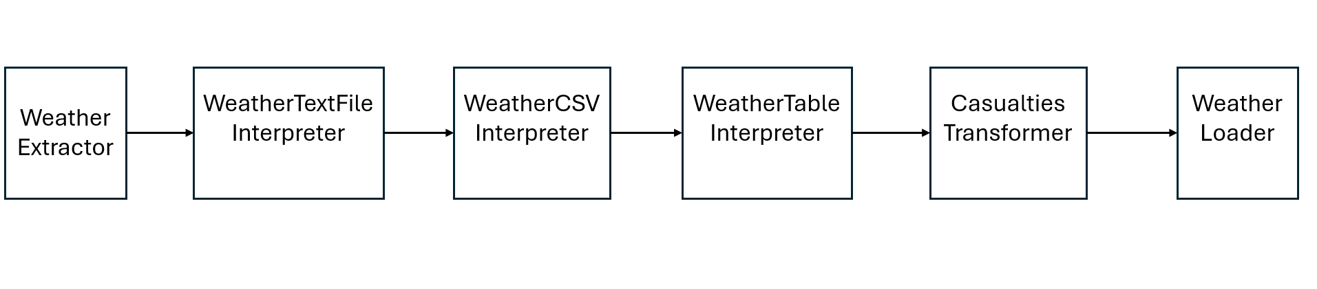
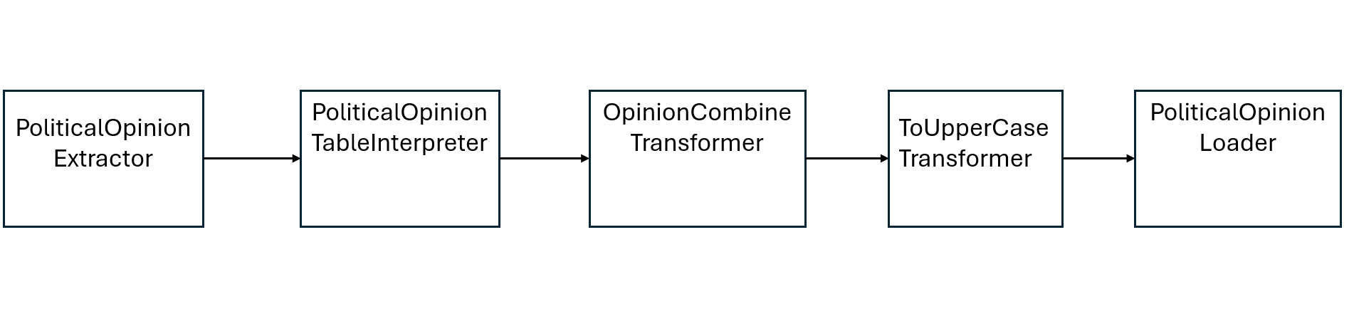
Lastly, the following figures summarize the pipelines:
Conclusion
In this post, we walked through the complete ETL process using a practical example built with the domain-specific language Jayvee. We saw how to extract data from both local files and online sources, how to transform it to clean and structure it for analysis, and finally how to load it into a format suitable for further use, such as a SQLite database.
We explored key transformation concepts – from filtering rows and selecting relevant columns, to formatting and computing new values. We also saw how to enforce data constraints and unify formatting, ensuring consistency and reliability in the resulting dataset.
Along the way, we learned why DSLs like Jayvee can be a powerful middle ground: more accessible than general-purpose programming languages, yet more scalable, and version-controlled than some no-code or visual tools.
Stay tuned for the next post, where we’ll go one step further – analyzing and visualizing the cleaned datasets to uncover insights on climate change impacts and public opinion trends.
AI Disclaimer
During the preparation of this work the author, as a non-native speaker, used LanguageTool and ChatGPT in order to improve wording, grammar and spelling. After using these tools, the author reviewed and edited the content as needed and takes full responsibility for the content.